2. Basic Usage
2.1. Plotting visibilities
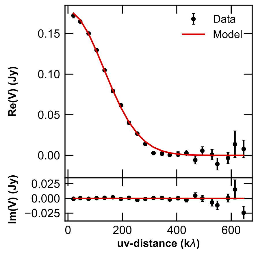
This is an example plot created with uvplot:
import numpy as np
from uvplot import UVTable, arcsec
from uvplot import COLUMNS_V0       # use uvplot >= 0.2.6

wle = 0.88e-3         # Observing wavelength         [m]

dRA = 0.3 * arcsec    # Delta Right Ascension offset [rad]
dDec = 0.07 * arcsec  # Delta Declination     offset [rad]
inc = np.radians(73.) # Inclination    [rad]
PA = np.radians(59)   # Position Angle [rad]

uvbin_size = 30e3     # uv-distance bin [wle]

uv = UVTable(filename='uvtable.txt', wle=wle, columns=COLUMNS_V0)
uv.apply_phase(dRA, dDec)
uv.deproject(inc, PA)

uv_mod = UVTable(filename='uvtable_mod.txt', wle=wle, columns=pluCOLUMNS_V0)
uv_mod.apply_phase(dRA=dRA, dDec=dDec)
uv_mod.deproject(inc=inc, PA=PA)

axes = uv.plot(label='Data', uvbin_size=uvbin_size)
uv_mod.plot(label='Model', uvbin_size=uvbin_size, axes=axes, yerr=False, linestyle='-', color='r')

axes[0].figure.savefig("uvplot.png")
From version v0.2.6 it is necessary to provide the columns parameter
when reading an ASCII uvtable. The columns parameter can be specified
either as a parameter to the UVTable() command, or as the 2nd line
in the ASCII file. The available columns formats are:
FORMAT          COLUMNS                                                 COLUMNS_LINE (copy-paste as 2nd line in the ASCII file)
COLUMNS_V0      ['u', 'v', 'Re', 'Im', 'weights']                       '# Columns      u v Re Im weights'
COLUMNS_V1      ['u', 'v', 'Re', 'Im', 'weights', 'freqs', 'spws']      '# Columns      u v Re Im weights freqs spws'
COLUMNS_V2      ['u', 'v', 'V', 'weights', 'freqs', 'spws']             '# Columns      u v V weights freqs spws'
To import an ASCII uvtable with 5 columns with uvplot < 0.2.6:
from uvplot import UVTable
uvt = UVTable(filename='uvtable.txt', format='ascii')
and with uvplot >= 0.2.6:
from uvplot import UVTable
from uvplot import COLUMNS_V0  # ['u', 'v', 'Re', 'Im', 'weights']
uvt = UVTable(filename='uvtable.txt', format='ascii', columns=COLUMNS_V0)
2.2. Exporting visibilities from MS table to uvtable (ASCII)
Once installed uvplot inside CASA (see instructions above),
it is possible to export the visibilities in mstable.ms to an ASCII table by executing these lines from a CASA shell:
CASA <1>: from uvplot import export_uvtable
CASA <2>: export_uvtable("uvtable.txt", tb, vis='mstable.ms')
Note: it is strongly recommended to perform a CASA split command with keepflags=False before exporting the uvtable. This ensures that only valid visibilities are exported.
The resulting uvtable.txt will contain u, v coordinates (in meters), Re(V), Im(V) visibility measurements (in Jansky),
and weights. The table will also report the average wavelength (averaged among all selected spectral windows):
# Extracted from mstable.ms.
# wavelength[m] = 0.00132940778422
# Columns:  u[m]    v[m]    Re(V)[Jy]       Im(V)[Jy]       weight
-2.063619e+02       2.927104e+02    -1.453431e-02   -1.590934e-02   2.326950e+04
3.607948e+02        6.620900e+01    -1.680727e-02   1.124862e-02    3.624442e+04
5.752178e+02        -6.299933e+02   5.710317e-03    6.592049e-03    4.719500e+04
-9.198434e+02       -1.374651e+03   1.313417e-03    4.299262e-03    4.259890e+04
9.623210e+01        -4.631573e+02   7.731462e-03    -8.803369e-03   4.801395e+04
9.348914e+01        -5.191096e+02   3.759772e-03    4.754967e-04    4.748304e+04
1.108410e+03        -1.396906e+03   3.222965e-03    -5.164917e-03   4.690977e+04
[...]
By default export_uvtable exports all channels in all spectral windows. However, it is also possible to specify which
spectral windows and channels to export. More details are given in the documentation of the export_uvtable() function.
Note: currently, export_uvtable only works for MS tables where all the spectral windows have the same number of channels (which, individually, can be larger than 1).